Statistics is all about data, particularly those quantitative information and even qualitative facts converted to numerical equivalents. So what is being done with these data? After collecting and organizing them, we summarize and present them in a simplified and compressed form that is easy to understand and discern. The much harder task is the interpretation of the results and of the summary you have made.
With regards to summarizing and presenting statistical data, the key activities are computation and creation of charts or tabular presentations. We can do it manually or using calculators. But with the bulk of data that you may have, such work would be difficult. However, Microsoft Excel can do the job with an eyes’ blink. It is a software program common to almost every computer and hence, this simple step-by-step tutorial can be followed by anyone.
In statistics, one way of summarizing data is to compute for the measures of central tendency (such as mean, median, and mode) and the measures of variation (such as standard deviation and variance). Here is a quick guide to computing them using Microsoft Excel.
First, install the add-on for statistical computing. This add-on is featured in all Microsoft Excel versions but is not yet activated. One must install it first. To do this, open Microsoft Excel (I am using 2007 version, but it also works for others).
Click Office Button.

Click Excel Options.

A menu box opens. Click Add-Ins (at the left bar). Then go to Manage (at the bottom), select Excel Add-Ins, and click the Go… button.

Another set of options opens. Check Analysis Toolpak and/or Analysis Toolpak – VBA.

Wait for the Add-on to be installed in your unit.
When it is done, you can observe that the Data Analysis command has been added to you Data menu. If you click that, you will be given options on what statistical computing you wish to do.

Let us solve the following sample problem with Mircosoft Excel.
Sample Problem: A random sample of students in a sixth grade class was selected. Their weights are given in the below. Summarize the data.
63 64 76 76 81
83 85 86 88 89
90 91 92 93 93
93 94 97 99 99
99 101 108 109 112
First thing to do is to encode the data on Microsoft Excel. See to it that data are in a single column or row.

Go to Data, and then Data Analysis. Look for the Descriptive Statistics. Click OK.

The Input Range requires you to specify the data you want to analyze. Click the icon beside (to the right) that and highlight the cells containing the data. Then click the same icon again to return to the command box.


To specify which particular cell you want the results to be shown, click the icon after Output Range. Select the location (say beside the data), and click the same icon again.

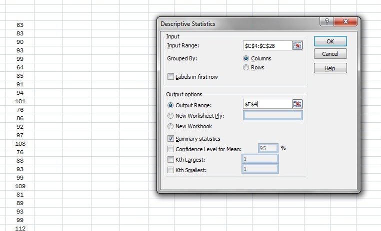
See to it that the Summary Statistics have been checked. Then click OK.

That’s it! Summary is immediately presented. It is just as easy as that.

There are still several statistical computations that you can do with Data Analysis. Once you have acquainted yourself with it, you can then explore and play around.
Follow this article at Factoidz.
Follow this article at Factoidz.
شركة نقل عفش
ReplyDeleteشركة نقل عفش بجدة
شركة نقل عفش بالطائف
شركة نقل عفش بالمدينة المنورة